Welcome to quantum mechanics 12, the Dirac equation. This is a video about an equation, and it will contain quite a bit of math, including review from previous videos as well as new material. Nonetheless, we’ll try to keep focused on physical concepts. The two revolutionary new theories of early 20th century physics were quantum mechanics and relativity. This series has traced the development of quantum mechanics. There is a companion series on relativity. In this video we investigate how quantum mechanics and special relativity can be combined to give a more complete theory of the electron. This leads to the Dirac equation, the equation of relativistic quantum mechanics for the electron. The Dirac equation explicitly requires spin as an intrinsic property of the electron. It gives improved values for hydrogen atom energy levels including the fine structure.

And, it predicted the existence of anti-matter before there was any reason to imagine such a thing. We only need a single equation from relativity. In video 9 of the relativity series we derived the famous relation E equals m c squared. This gives the intrinsic energy of a particle in terms of its rest mass m and the speed of light c. We showed that when the particle moves with velocity v its energy increases by a factor of one over square root 1 minus v over c squared. This can be expanded in a series of terms. The first term is the rest energy m c squared. The second term is the classical kinetic energy one-half m v squared.

This is multiplied by the series of terms in brackets which gives the relativistic correction to kinetic energy. Relativistic momentum is the classical value with the addition of the same square root expression. Eliminating v from these last two equations we can express energy as a function of particle momentum and mass as E equals square root of p-c squared plus m-c squared, squared. This is the equation we will use as a basis for relativistic quantum mechanics. As a check we see that for a particle with zero momentum this reduces to E equals m c squared. For a photon, which has zero rest mass, it reduces to E equals p c. As we saw in the video on photons, a photon with wavelength lambda has momentum Planck’s constant over lambda, and c over lambda equals frequency nu. Thus we obtain the Planck relation E equals h nu. Imagine some quantity u which varies through time t to define a curve u of t. At any point on the curve we can draw a right triangle through the point tangent to the curve. The ratio of the sides of this triangle is the slope of the curve at that point.

We can also draw a circle through the point which coincides with neighboring points on the curve. The inverse of the radius of this circle is the curvature of the curve at that point. In calculus notation we write the slope using two curly letter d’s which we call the derivative of u with respect to t. We’ll use the short-hand notation curly d with subscript t and refer to this as the slope in t of u. The curvature is the derivative of the derivative, or second derivative of u with respect to t. We’ll use the notation curly d squared with subscript t and refer to this as the curvature in t of u. A very important class of wave functions are the so-called plane waves. These have the form psi equals e to the i k x minus omega t where i is the imaginary unit, the square root of negative one. We can think of this as a short-hand for cosine of k x minus omega t plus i times sine of k x minus omega t. The time slope of psi is minus i omega psi while the x slope is i k psi.

The magnitude of psi is one everywhere, so this wave function represents a particle with a uniform probability of appearing anywhere at any time but with definite energy and momentum in the x direction. As time goes on the real, cosine part (in red), and the imaginary, sine part (in green) propagate in the x direction. In the video on angular momentum we discussed the concept of operators. The energy operator E hat is i h-bar slope in time. The x momentum operator, p-x-hat is minus i h-bar slope in x, and likewise for the y and z components of momentum. For a state of definite energy, the energy operator applied to the wavefunction gives the energy value times the wavefunction. Likewise for the three momentum operators. We also described non-commuting operators. If p-hat q-hat minus q-hat p-hat is not zero then applying these operators to a wavefunction in a different order will not give the same results.

It follows that we cannot simultaneously know, or measure, both p and q. Recall the definition of angular momentum. If a particle is at location (x,y,z) moving with momentum (p-x,p-y,p-z) the components of its angular momentum are (L-x,L-y,L-z). Taking the classical expressions and substituting momentum operators we obtain the angular momentum operators. These operators do not commute. Instead they satisfy the commutation relations shown here. Now for the new material. We’ve talked about electron spin in previous videos, but we haven’t given much thought to a rigorous representation of it. Let’s do that now. We picture a particle spinning about one of the two red axes such that the component of angular momentum along the z axis is either plus h-bar over two or minus h-bar over two. This is a spin one-half particle for which the quantum number m sub s can be either minus one-half or plus one-half.

We can know the magnitude of spin angular momentum, square-root of 3 over 2 h-bar, and the component along one axis, which we usually take to be the z axis, but not the other two components. Let’s assume spin is described by angular momentum operators s-hat x, s-hat y and s-hat z. We’ll abstractly represent the two states, spin up and spin down by Dirac kets with an up-arrow or down-arrow. Because the spin-up state is a state of definite angular momentum z-component, we must have that the s-hat z operator applied to the up state gives h-bar over 2 times the up state.

Similarly for the spin down state. A more concrete representation of spin takes the form of a two-component array or matrix. For spin up the upper component is one and the lower component is zero. For spin down this order is reversed. To represent a superposition of states we simply add the corresponding components. We define the product of a two-by-two matrix with components A, B, C and D and a two-by-one matrix with components u and v to be a two-by-one matrix with components A-u plus B-v and C-u plus D-v. If this two-by-two matrix represents the s-hat z operator then s-hat z times the spin up state has components A and C.

If this equals h-bar over 2 times the spin up state then A equals h-bar over 2 and C equals zero. Repeating for the spin down state we find B equals 0 and D equals minus h-bar over two. This gives us the s-hat z operator as h-bar over two times the two-by-two matrix with components 1, 0, 0, minus one. As shown here, the product of two, two-by-two matrices is another two-by-two matrix. We assume the spin operators satisfy the normal angular momentum operator commutation relations. Representing the s-hat x and s-hat y operators by matrices with unknown elements, we can solve the commutation relations for those unknown values to obtain the representations shown here. It’s convenient to define versions of these without the h-bar over two factors.

These are known as the Pauli matrices after Wolfgang Pauli who played a central role in developing the concepts and mathematics of electron spin. The spin operators are then h-bar over 2 times the Pauli matrices. Let’s use these ideas to develop a representation of an electron wave function that includes spin. Up to now we’ve simply taken a spin-less wave function and added a factor to represent spin up, or spin down. With our matrix notation we can put the wave function in the spin up position, or in the spin down position. An arbitrary spin state can be represented by having different wave functions, psi 1 and psi 2, as the spin up and spin down components.

We call this form of wavefunction a spinor. The magnitude squared of psi 1 gives the probability that the electron is at some point, at some time, with spin up. The magnitude squared of psi 2 gives the probability that the electron is at some point, at some time, with spin down. The power of this representation is that it allows the probability of spin up or down to vary with time and position as could be the case if time and space-varying magnetic fields are present. At a given time the total probability that the electron is somewhere in space with some spin is one. Let’s now try to develop a relativistic wave equation. We start with the relativistic expression for energy. Substituting energy and momentum operators, and applying the operators on both sides to a wave function gives us this expression. Here the Laplacian symbol is a short-hand for the sum of the spatial curvatures. This is problematic, because it’s not clear what the square root of an operator even means, how to apply it, or how to solve an equation containing it.

One way forward is to square both sides of the energy equation. We then have E squared equals p-c squared plus m-c-squared, squared. Now we substitute operators and apply both sides to a wave function. Eye h-bar squared is minus h-bar squared. Two slope-in-time operators give the curvature in time operator, and on the right side we no longer have the square root of an operator. This is the Klein-Gordon equation. There are some problems with applying this equation to the electron, however. Because we started with an expression for the square of energy, the energy itself can be either positive or negative. For every positive energy solution there will be a negative energy solution. Negative energy seems unphysical. The equation gives us the curvature in time of the wave function, unlike the Schr�dinger equation that gives us the slope in time.

Mathematically to solve for future states of the system we need to specify both the wave function and the slope of the wave function at some initial time. This isn’t in the spirit of the idea that the wave function itself fully specifies the state of a system. It’s not possible to maintain the interpretation of the magnitude squared of the wave function as a probability of finding the electron at some point. In fact, the sum of this over all space isn’t even necessarily constant.

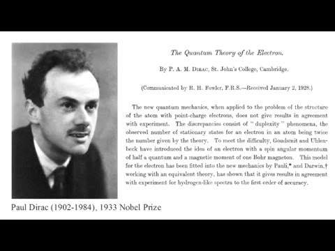
When applied to the hydrogen atom this equation predicts incorrect energy levels, which is obviously a step down from the success of the Schr�dinger equation. And there is nothing in the solution of the equation that would require or predict electron spin. In fact, it turns out that the Klein-Gordon equation describes the behavior of spin-less particles. In 1928 Paul Dirac presented a new equation of relativistic quantum mechanics that sought to overcome these problems. To simplify our expressions we use so-called natural units in which c and h-bar are one. Then our formula for E reduces to the square root of p squared plus m squared. Dirac’s idea was to try and express this as a sum of four terms in p-x, p-y, p-z and mass. Here the alphas and beta are four unknown constants. To determine these constants we square both sides to get E squared equals p squared plus m squared equals the product of this four-term expression with itself. Each of the four terms in the first factor will appear in a product with each of four terms in the second factor, so there will be a total of 16 terms in all.

Four of those will be the product of a term with itself, such as alpha-x p-x times alpha-x p-x, and this results in the four squared terms shown here. What remains are 12 cross-terms, such as alpha-x p-x times alpha-y p-y and alpha-y p-y times alpha-x p-x. Adding those 12 cross-terms we get the full expression for E squared. Now, this must equal p squared plus m squared. p squared is related to the components of momentum by the Pythagorean theorem, p-x squared plus p-y squared plus p-z squared. Comparing these expressions it’s clear that we need all the cross terms to go away and the squares of the four constants to be one. Consider the cross terms alpha-x alpha-y p-x p-y plus alpha-y alpha-x p-y p-x.

The p-hat-x and p-hat-y operators commute with each other. We can know all three components of linear momentum. So p-y p-x equals p-x p-y and we are justified in factoring out the momentum terms. To make this expression zero we need the constant in parentheses to vanish. So alpha-x alpha-y must equal minus alpha-y alpha-x. If the alphas are numbers this can only be true if at least one of them is zero. But we need the square of each of these to be one, so there is no solution. However, Dirac realized that a solution could exist if the alphas are matrices. In fact, the Pauli matrices satisfy just such relations. Each pair anti-commute, and the square of each equals a two-by-two identity matrix. The product of the identity matrix and a spinor is the spinor. So the identity matrix is the matrix equivalent of the number one. What appeared to be a bug in this approach seems like it may instead be a feature.

This equation may explicitly involve spin operators implying that spin is an intrinsic requirement of a relativistic theory of the electron. Unfortunately we need four such matrices, three alphas and a beta. There are only three Pauli matrices and it’s not possible to find four two-by-two matrices satisfying our requirements. It is possible, however, to find four, four-by-four matrices that solve our problem. Dirac’s matrices are shown here. Notice that each of the alphas contains two copies of the corresponding Pauli matrix, and beta contains two, two-by-two identity matrices, one being negated. Taking this solution and substituting energy and momentum operators we arrive at the desired equation.

The Dirac equation for a free electron. Consider one of these terms, say the m-beta-psi term. If beta was a two-by-two matrix then we’d expect psi to be a two-component spinor. But beta is a four-by-four matrix, so psi has to have four components, one for each column of beta, in order for the matrix multiplication to make sense. Using a wave function of this form and carrying out the matrix multiplications, Dirac’s equation takes the form shown here. This actually represents four separate equations in the four wave function components psi 1, 2, 3 and four. If psi was a two-component spinor we could readily interpret one component as corresponding to spin up and the other to spin down. But what are we to make of a four component object? We need to find solutions to these equations and then try to determine if this type of wave function corresponds to something real or if it is just another dead-end on our quest for a relativistic wave equation of the electron..